Kyushu University Faculty of Science

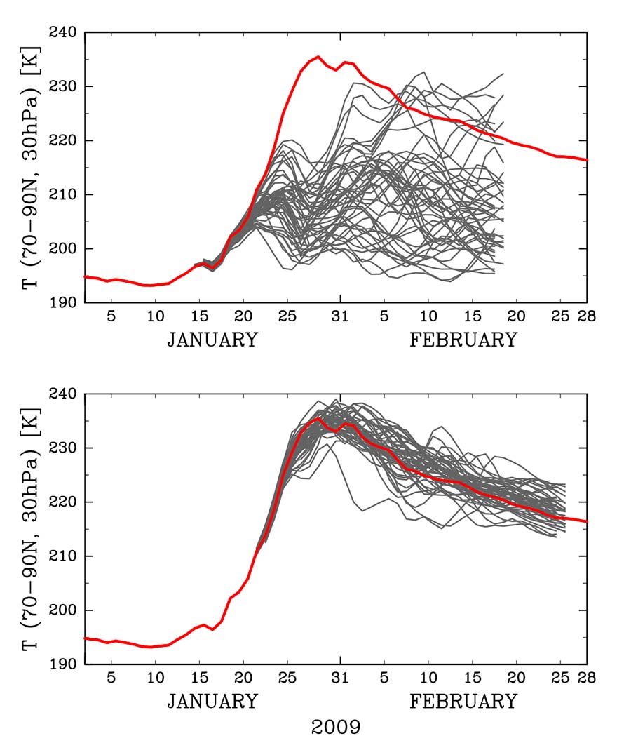
In the middle atmosphere, a unique phenomenon called “stratospheric sudden warming” (SSW) sometimes occurs, in which the temperature in the polar stratosphere rapidly rises over a few dozen degrees Kelvin within several days, a situation unimaginable in the troposphere. Figure 1 shows the time series of the stratospheric temperature over the Arctic for one winter, with observed values (red line) and predicted values (thin black lines). It illustrates the results of multiple predictions starting from slightly different initial conditions (i.e., ensemble forecasts). The observations indicate an SSW from mid to late January. The ensemble forecast initiated well before the event (upper panel) fails to capture the peak of SSW and shows a large spread among ensemble members. In contrast, all ensemble members in the forecast initiated just before the event (lower panel) accurately reproduce the warming evolution. Therefore, from this point, we could reliably predict the time evolution of this SSW. Investigating how these variations in forecast characteristics (i.e., predictability variations) are related to flow features and how they impact predictions in other regions is an important research topic.

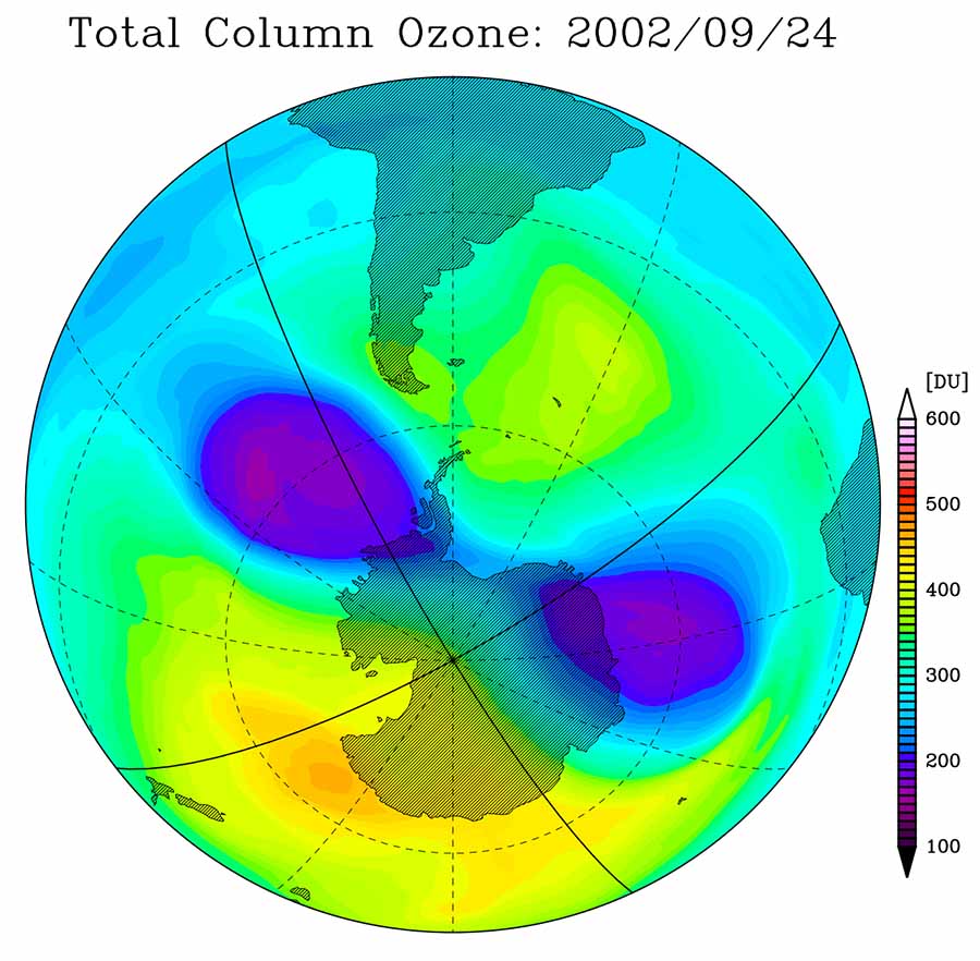
The middle atmospheric circulation is shaped by close interactions between dynamics, radiation, and chemistry. Figure 2 shows the temporary shrinking of the ozone hole, which had been developing to cover the entire Antarctic continent every spring since the 1980s, when it split into two (a very rare condition) by atmospheric dynamical variations. This example provides a suitable situation for investigating interactions with atmospheric chemistry and radiation. How does such a large-scale flow change affect material circulation and subsequently atmospheric composition? Conversely, how much do changes in atmospheric composition and radiative forcing alter the flow? By quantitatively elucidating the strength of interactions among the components of the Earth system, we can gain a more detailed understanding of the Earth's environment.

Rotation and sphericity of the Earth affect the motion of the air or water on it in a number of aspects. Figure 3 illustrates the flow driven by a localized warm water pool of Amazon size placed at the equator. We see complex structure of wind change emerge all over the globe. This result is obtained in an idealized earth, all covered with ocean, on which we see the character of flow on rotating spherical planet more clearly than on the Earth which has many complex features like continent and mountains.

When flowing up or down in a large distance, due to the change of temperature or pressure, the phase change of material occurs in the fluids, resulting in the formation of cloud and rain. Everybody knows those on the Earth, but clouds and rain develop also in the atmospheres of planets and its satellites. Figure 4 shows lightning in the thunderstorms of Jupiter's atmosphere. Cumulonimbus clouds of methane develop in the atmosphere of Titan, the largest satellite of Saturn. There are many poorly known issues on these extraterrestrial clouds.